Numerical Methods 2: Analysis of chaotic behavior in nonlinear equations with animation techniques
Goal:
Understanding
- Numerical analysis of Lorenz Equation as a model which shows chaotic motions
- GUI for setting parameters
- method for creating animation
In the previous section, we numerically solved nonlinear differential equations for two variables. Their trace approaches a fixed point or a limit cycle, which is called a "simple" attractor.
In this section, we will investigate three-variable equations which exhibit more complex behavior where the attractor is complex one called "strange attractor".
Nonlinear differential equations with unstable trajectory
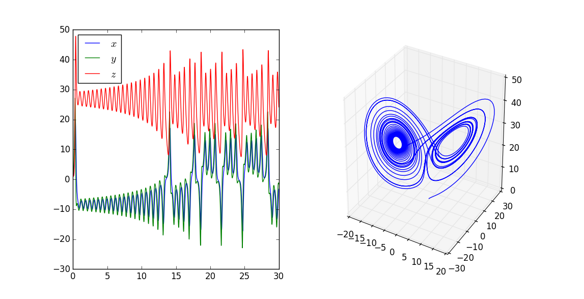
Some dynamical equations with variables whose number is larger than 3 are known to show a complex trajectory. Those are called "Chaos". A most welknown equation is Lorenz equation defined by $$ \begin{eqnarray} \frac{dx}{dt} &= \sigma (y-x) \\ \frac{dy}{dt} &= -xz + rx - y\\ \frac{dz}{dt} &=xy -bz \end{eqnarray} $$ where $(x(t), y(t), z(t))$ are time-dependent variables and $\sigma,\ r,\ b$ are constants. This equation was derived by Lorenz in the early 60s. His goal was to describe the motion of atomospheric convection on the earth surface and reduced the degrees of freedom of the fluid equation to 3 variables.
The trajectory falls into a complex plane called "strange attractor" of which shape is like a butterfly . The plane is very thin (thickness is zero) but the trajectory never cross a point because the equation is deterministic and it is not periodic. Analytical study shows this attractor has the fractal dimension 2.06 (not integer, 2).
A movie made by a python code using animation library is shown here. (The code is shown at the bottom of this notebook.) You can also find many examples by searching by keywords like "lorenz attractor python" on the Web.
Exercise 2-1
Soluve numerically the above equation and show the trajectory on a graphic plane and plot the values of 3 variables versus time.
Sensitivity to the initial difference
One of remarkable characterisics of chaos is the sensitivity to the initial values. To see this, try to trace two trajectories with a small difference at the initial states.
Try to execute the following code by changing the parameters.
from scipy import spatial as sp
import numpy as np
from scipy import integrate
import matplotlib.pyplot as plt
from mpl_toolkits.mplot3d import Axes3D
import math

def lorentz_deriv(x, t0, sigma=10., beta=8./3., rho=28.0):
    """Compute the time-derivative of a Lorenz system."""
    return (sigma * (x[1] - x[0]),
            x[0] * (rho - x[2]) - x[1],
            x[0] * x[1] - beta * x[2])

def calc_and_plot_2ini(sigma, beta, rho, max_time=20, diff_ini=-4, run=True) :
    '''
    The difference of z value between initial conditions is given by the power 1.**diff_ini
    '''

    if not run:
        return "not run"

    x0 = [1., 1., 1.]  # starting vector
    x1 = [1., 1., 1.+ 10.**diff_ini]

    t = np.linspace(0, max_time, max_time*100) # time step is fixed
    x_t = integrate.odeint(lorentz_deriv, x0, t, args=(sigma, beta, rho))
    x1_t = integrate.odeint(lorentz_deriv, x1, t, args=(sigma, beta, rho))

    fig =plt.figure(figsize=(12,5))

    ax1= fig.add_subplot(1,2,1,projection='3d')  # Axes3D is required
    ax1.plot(x_t[:,0], x_t[:,1], x_t[:,2])
    ax1.plot(x1_t[:,0], x1_t[:,1], x1_t[:,2])
    plt.title('$\sigma =' + str(sigma) + '$, $\\beta =' + str(beta)
              + '$, $\\rho =' + str(rho) + '$')

    ax2 = fig.add_subplot(1,2,2) # plotting the expansion of the two traces
    dist = [math.log10(np.linalg.norm(x_t[i,:] -x1_t[i,:]))
            for i in range(t.size)] # distance between 2 traces
    ax2.plot(t,dist)
    ax2.set_xlabel("$t$")
    ax2.set_ylabel("$\log_{10}\Delta$ (distance in log scale)")

    plt.show()

from ipywidgets import interact, interactive, Checkbox
from IPython.display import clear_output, display, HTML

interact(calc_and_plot_2ini, sigma=(0.0,20.0), beta=(0, 8.0), rho=(0.0, 40.0),
         max_time=(10,50,1), diffIni=(-8,0,1), run=Checkbox(value=False))
If you user "interact_manual" instead of "interact", the function given as the 1st argument run after pressing "Run Interact".
def calc_and_plot_2ini(sigma, beta, rho, max_time=20, diff_ini=-4) :
    '''
    The difference of z value between initial conditions is given by the power 1.**diff_ini
    '''

    x0 = [1., 1., 1.]  # starting vector
    x1 = [1., 1., 1.+ 10.**diff_ini]

    t = np.linspace(0, max_time, max_time*100) # time step is fixed
    x_t = integrate.odeint(lorentz_deriv, x0, t, args=(sigma, beta, rho))
    x1_t = integrate.odeint(lorentz_deriv, x1, t, args=(sigma, beta, rho))

    fig =plt.figure(figsize=(12,5))

    ax1= fig.add_subplot(1,2,1,projection='3d')  # Axes3D is required
    ax1.plot(x_t[:,0], x_t[:,1], x_t[:,2])
    ax1.plot(x1_t[:,0], x1_t[:,1], x1_t[:,2])
    plt.title('$\sigma =' + str(sigma) + '$, $\\beta =' + str(beta)
              + '$, $\\rho =' + str(rho) + '$')

    ax2 = fig.add_subplot(1,2,2) # plotting the expansion of the two traces
    dist = [math.log10(np.linalg.norm(x_t[i,:] -x1_t[i,:]))
            for i in range(t.size)] # distance between 2 traces
    ax2.plot(t,dist)
    ax2.set_xlabel("$t$")
    ax2.set_ylabel("$\log_{10}\Delta$ (distance in log scale)")

    plt.show()

from ipywidgets import interact_manual
interact_manual(calc_and_plot_2ini, sigma=(0.0,20.0), beta=(0, 8.0), rho=(0.0, 40.0),
         max_time=(10,50,1), diffIni=(-8,0,1))
As you can see in the above simulation, The difference at the initial state expands exponentially. Such an exponential behavior means that the future is determined but eventually unpredictable. (このような系は、未来は決定されているが予測不可能であるという。)
3D animation of Lorenz equation
The point is:
- cretate figure object of matplotlib
- define update function of the trajectory updated by the Lorenz eq.
- give the definition to the animating function, "animation.FuncAnimation"
If you install "ffmpeg" library, you can save the animation to a mpeg4 movie file.
# coding: UTF-8
"""
Lorenz model visualization as an exercise on animation
    continue to plot until the run quits.
"""
%matplotlib auto

import numpy as np
from scipy import integrate
from matplotlib import pyplot as plt
from mpl_toolkits.mplot3d import Axes3D
from matplotlib import animation

def lorentz_deriv(x, t0, sigma=10., beta=8./3, rho=28.0):
    """
    Compute the time-derivative of a Lorentz system.
    draw two trajectories with a tiny difference between them: x_ini1, x_ini2

    """
    return [sigma * (x[1] - x[0]), x[0] * (rho - x[2]) - x[1], x[0] * x[1] - beta * x[2]]

# Create new Figure and an Axes which fills it.
fig = plt.figure()
ax = fig.add_axes([0, 0, 1, 1], projection='3d')
# prepare the axes limits
ax.set_xlim((-25, 25))
ax.set_ylim((-35, 35))
ax.set_zlim((5, 55))

# set point-of-view: specified by (altitude degrees, azimuth degrees)
# ax.view_init(60, 45)

# initial setting
t = np.linspace(0,0.1,10)

x_ini1 = [1., 1., 1.]  # starting vector:  two traces with different initial value
x_ini2 = [1.00001, 1., 1.]

line1, = ax.plot([], [], [], 'b-')
line2, = ax.plot([], [], [], 'r-')
pt1, = ax.plot([],[],[], 'bo')
pt2, = ax.plot([],[],[], 'ro')

data4plot1 = integrate.odeint(lorentz_deriv, x_ini1,t)
data4plot2 = integrate.odeint(lorentz_deriv, x_ini2,t)

#update
def update(i) :
    global x_ini1, x_ini2, x_t, line1, line2, data4plot1, data4plot2
    # update the trajectory from x_ini1
    x_t = integrate.odeint(lorentz_deriv, x_ini1,t)
    data4plot1 = np.vstack((data4plot1, x_t)) # add the current point to the trajectory
    line1.set_data(data4plot1[:,0],data4plot1[:,1])
    line1.set_3d_properties(data4plot1[:,2])  # show the trajectory
    pt1.set_data(data4plot1[-1:,0], data4plot1[-1:,1])    # head (current point)

    pt1.set_3d_properties(data4plot1[-1:,2])
    x_ini1 = x_t[-1]                          # initial values for the next step

    # update the trajectory from x_ini2
    x_t = integrate.odeint(lorentz_deriv, x_ini2,t)
    data4plot2 = np.vstack((data4plot2, x_t))
    line2.set_data(data4plot2[:,0],data4plot2[:,1])
    line2.set_3d_properties(data4plot2[:,2])
    pt2.set_data(data4plot2[-1:,0], data4plot2[-1:,1])    # head (current point)

    pt2.set_3d_properties(data4plot2[-1:,2])
    x_ini2 = x_t[-1]                          # initial values for the next step


    ax.view_init(30, 0.3 * i)   # rotating eye's point
    fig.canvas.draw()

# Construct the animation, using the update function as the animation
# director.
anim = animation.FuncAnimation(fig, update,
                               frames=300, interval=10)
# To make movie file, use anim.save function like the below line
# anim.save('lorentz3d.mp4', fps=15, extra_args=['-vcodec', 'libx264'])

# To make movie as a moving "gif" file, use the below (this will be huge)
# anim.save('lorentz3d.gif', writer='imagemagick',  fps=30)

plt.show()
Poincare map (Exercise 2-2 (optional))
To characterize the complex behavior of unstable trajectories such as Lorenz equation, Poincare map is useful. Poincare map is to make a discrete sequence of a variable picked up from a trajectory by a definite rule. Here, let's try to find peak values of $z$ and plot $n$th peak value $z_n$ versus $(n+1)$th peak $z_{n+1}$. You will get a plot as below.
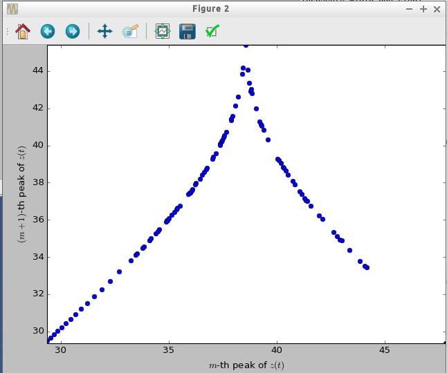
If the orbit is periodic, the Poincare map created by an initial condition yields some finite points: the number of points means the periodicity. On the contrary, the Poincare map of the Lorenz equation shows a continuous line with a steep top.
the Logistic Map which causes a complex behavior including bifurcation and chaos (optional)
The above figure is similar with a discrete map such as "Logistic Map" which shows a chaotic behavior accompanied with period-doubling bifurcation phenomena.
Logistic map is defined by $$ x_{n+1} = ax_n(1-x_n) $$
Let's plot $x_{n+1}$ versus $x_{n}$, which yields a figure as below.
%matplotlib inline
# Logistic map

import numpy as np
import matplotlib.pyplot as plt
def logisticFunc(xin,a):
    return a*xin*(1-xin)

a_vals = [1.5, 2.8, 3.3, 3.5, 3.7, 3.9]

x = np.arange(0,1.0,0.01)
fig = plt.figure(figsize=(14,9))
for i in range(6):
    axes = fig.add_subplot(2,3,i+1)
    a = a_vals[i]    # The parameter of the logistic map. Try to change the value between 0 < a < 4
    xn = 0.1   # initial value of the variable

    axes.plot(x, a*x*(1-x), 'r')
    axes.plot(x, x, 'k')
    axes.set_xlabel("$x_n$")
    axes.set_ylabel("$x_{n+1}$")
    axes.set_title("a=" + str(a))

    xnext = logisticFunc(xn,a)
    axes.plot([xn,xn],[0,xnext])
    for i in range(20):
        axes.plot([xn,xnext],[xnext,xnext],"b")
        xn = xnext
        xnext = logisticFunc(xn,a)
        axes.plot([xn,xn], [xn,xnext],"b")

plt.show()
As seen in the above figure, the tragectory asymptotically approaches a fixed point for $a=1.5$ and $a=2.8$, a 2-period fixed point for $a=3.3$, and a 4-period fixed point for $a=3.5$ whereas the case for $a=3.9$ looks a non-periodic complex trajectory.
The next figure shows the values of $x_n$ plotted on a vertical line for each $a$ after a transient regime. You can see the "period-doubling bifurcation" of the fixed point and chaotic regions between them. Not that the sequence of period.
If you execute the below code, you can plot this figure. If you have time, try to make a code that can yields a plot for arbitrary range of $x$ and $a$. The package "Tkinter" is used to plot the figure and utilize the control panel. If you wish to run in the "Wakari", you need to change "Anaconda" environment to be able to use this package (but I don't know whether it is possible.) If you are interested in running it in Wakari, please try it or you try to realize the same calculation by using matplotlib.
Some improved GUI programs for the Logistic map are shown in this page.
#  Derived from
#   chaos-3.py
#
#  Build Feigenbaum Logistic map. Input start and end K
#
#  python chaos-3.py 3.4 3.9
#
from Tkinter import * #Tk, Canvas, Frame, Button, Scale

canWidth=500
canHeight=500

def restartApp (ev) :
    global k1,k2, set_k1, set_k2
    canvas.create_rectangle(0, 0, canWidth, canHeight, fill = 'white')
    k1 = set_k1.get()
    k2 = set_k2.get()
    startApp()

def startApp () :
    global win, canvas, k1, k2
#   import sys

    x = .8                     # initial value of the map, which is somewhat arbitrary
    transient_range = range(50)
    vrng = range(300)          # We'll do 200 horz steps
    for t in range(canWidth) :
        win.update()
        k = k1 + (k2-k1)*t/canWidth
        # print "K = %.04f" % k
        for i in transient_range :
            x = x* (1-x) * k               # transient region is not drawn

        for i in vrng :
            p = x*canHeight
            canvas.create_line(t,p,t,p+1)  # just makes a pixel dot
            x = x * (1-x) * k              # next x value
            if x <0 or x >= 1.0 :
                print "overflow at k", k
                return

def setupWindow () :
    global win, canvas, set_k1, set_k2, k1, k2
    k1  = 3.5 # starting value of K
    k2  = 3.9   # ending   value of K

    win = Tk()

    # controler
    controlBox = Frame(win)
    StartBtn = Button(controlBox,text=u"restart", width=20)
    StartBtn.bind("<Button-1>", restartApp)

    # sliders for parameter setting
    set_k1 = Scale(controlBox, from_=1.0, to=3.9, resolution=0.1, orient=HORIZONTAL, labe="min")
    set_k2 = Scale(controlBox, from_=1.2, to=3.9, resolution=0.1, orient=HORIZONTAL, labe="max")
    set_k1.set(k1) # initial value
    set_k2.set(k2)
    canvas = Canvas(win, height=canHeight, width=canWidth)

    # Drawing frame
    f = Frame (win)
    canvas.pack(side="left")
    StartBtn.pack()
    set_k1.pack()
    set_k2.pack()
    controlBox.pack(side="right")
    f.pack()

if __name__ == "__main__" :
    setupWindow()       # Create Canvas with Frame
    startApp()          # Start up the display
    win.mainloop()      # Just wait for user to close graph
Making animations
Some example codes are shown in this notebook.
The following are the movies created by the examples (try to click the play button in the "Out" part. This is also an example code to display a movie file in the notebook if you place the mp4 file in the "image" folder. The movie files can be downloaded from the links: lorenz_xyz_t.mp4 lorenz3d.mp4
import io
import base64
from IPython.display import HTML

video = io.open('images/lorenz_xyz_t.mp4', 'r+b').read()
encoded = base64.b64encode(video)
HTML(data='''<video alt="test" controls>
                <source src="data:video/mp4;base64,{0}" type="video/mp4" />
             </video>'''.format(encoded.decode('ascii')))
import io
import base64
from IPython.display import HTML

video = io.open('images/lorenz3d.mp4', 'r+b').read()
encoded = base64.b64encode(video)
HTML(data='''<video alt="test" controls>
                <source src="data:video/mp4;base64,{0}" type="video/mp4" />
             </video>'''.format(encoded.decode('ascii')))