多項式曲線フィッティング (2) 過学習を防ぐ「正則化」項
"IPython Interactive Computing and Visualization Cookbook" (O'Reilly, 2018)のサンプルプログラム8.1を例に (現在、原文はhttps://ipython-books.github.io/ にて閲覧できる。)
模式図はPRMLより。
2乗誤差最小化 (復習)
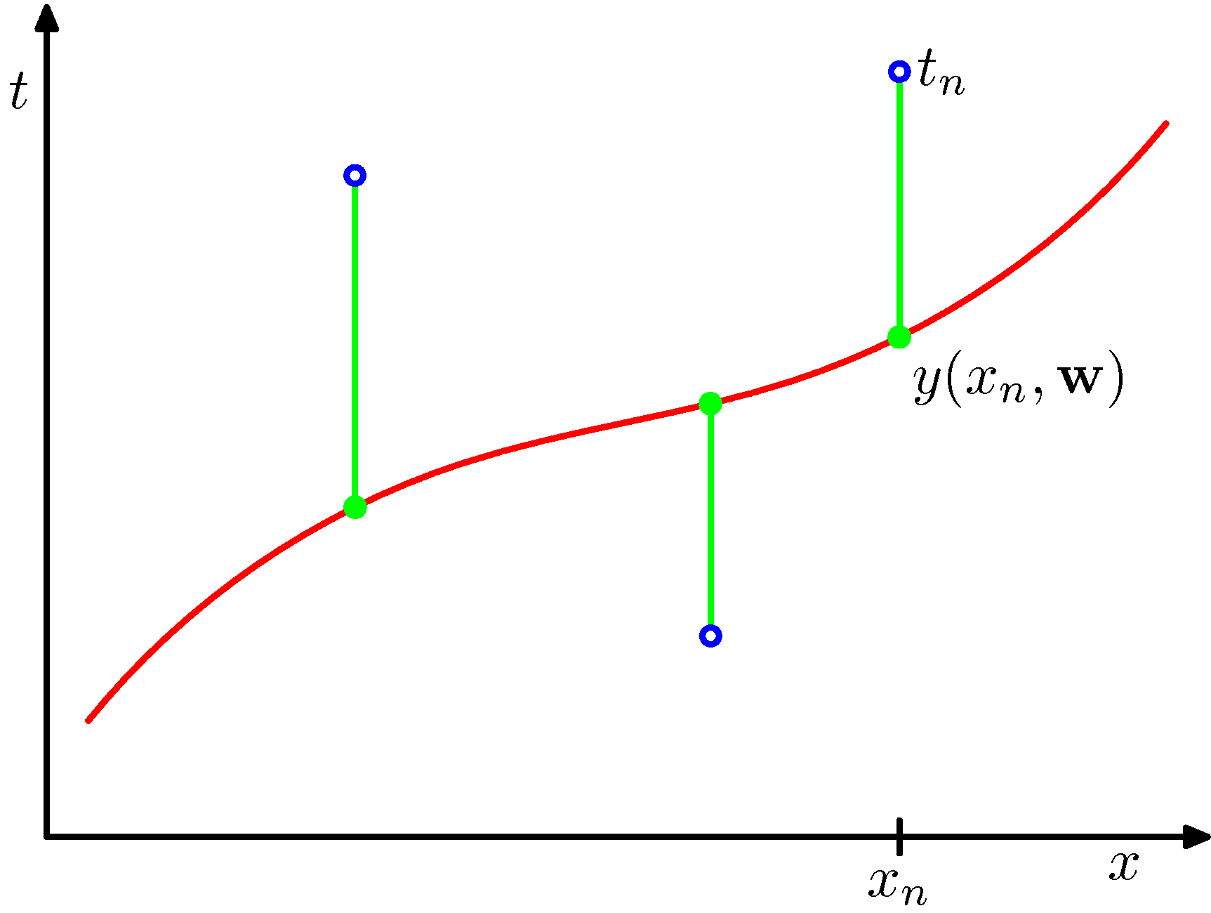
説明変数$x$に対する目的変数$y$について、$M$次関数でのフィッティングを考える: $$ y(x, {\bf w}) = w_0 + w_1 x + w_2 x^2 + \cdots + w_M x^M = \sum_{j=0}^{M} w_j x^j $$ データ$\{(x_n, t_n)\}$ ($n=1,\cdots N$)があったときに、 2乗誤差 $$ E({\bf w}) = \frac{1}{2} \sum_{n=1}^N \{y(x_n,{\bf w}) - t_n\}^2 $$ を最小にするよう${\bf w}$を決める。
説明用に、PRMLに載っている図を載せておく。
最小2乗法の模式図:
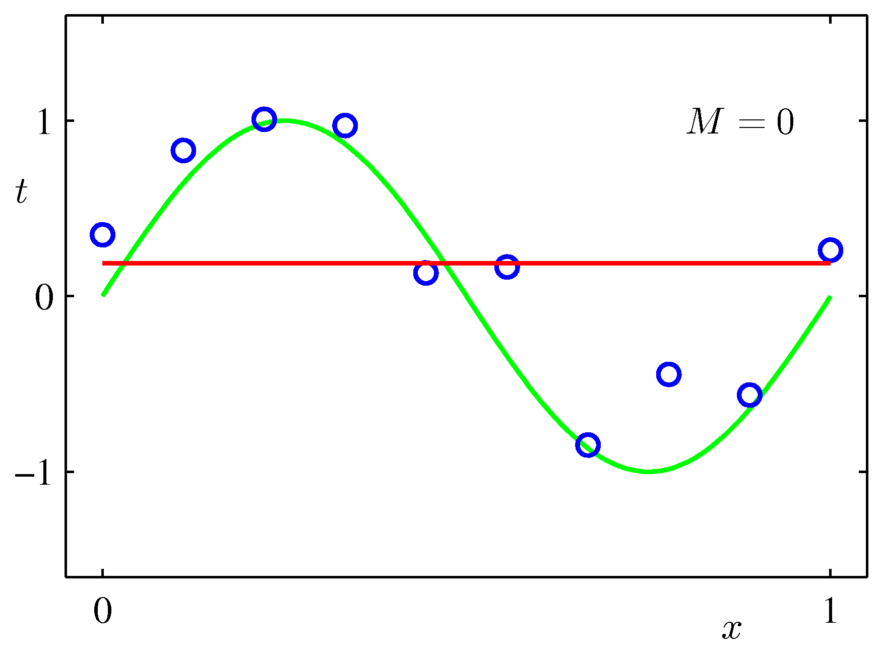
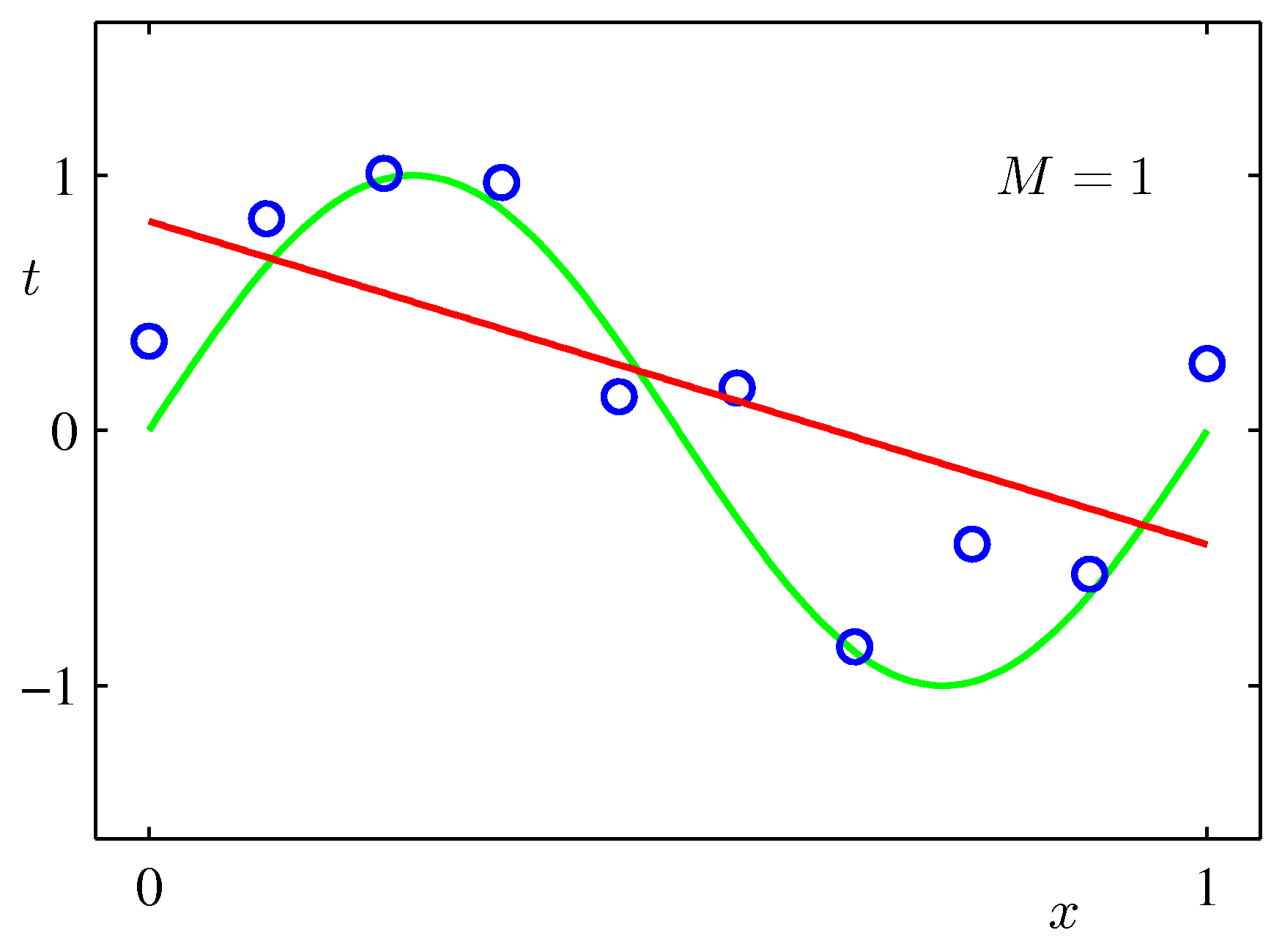
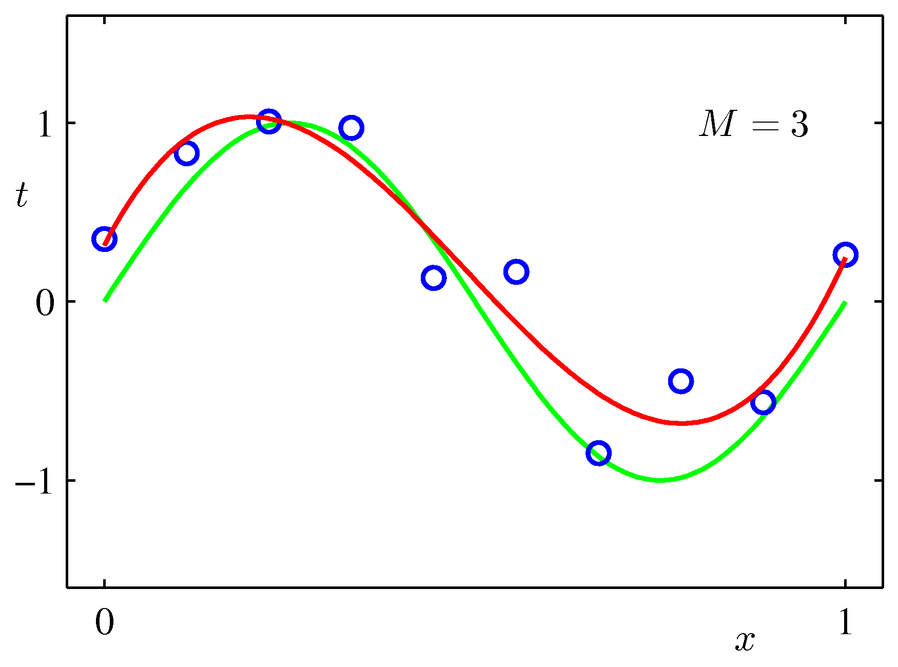
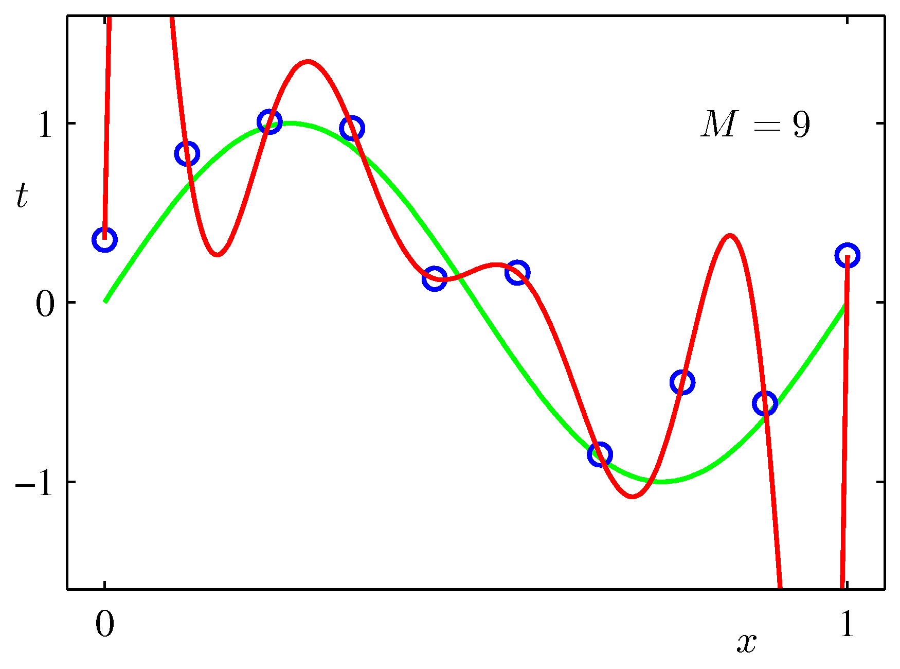
$\sin$カーブにノイズを載せたテストデータをべき関数フィッティングしてみた例:次数$M$をが大きいほうが全データにあうフィッティングができるが、不自然であることがわかるだろう。($M$が次数)
リッジ回帰
過学習を防ぐために、次のような係数に対する2次関数を付加し、その最小化を図る。この項は大きな係数の方が不利になるので、高次の項の「暴発」が抑えられる。
$$ \tilde{E}({\bf w}) = \frac{1}{2} \sum_{n=1}^N \{y(x_n,{\bf w}) - t_n\}^2 + \frac{\lambda}{2}||{\bf w}||^2 $$これはリッジ回帰(ridge regression)を呼ばれる。ニューラルネットでは、過重減衰(weight decay)として知られている。
また、このことを正則化(regularization)と呼ぶ。
リッジ回帰における重み係数
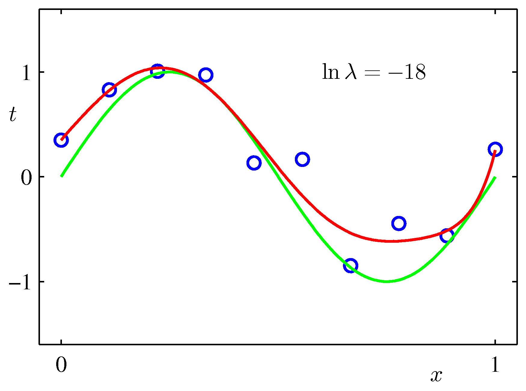
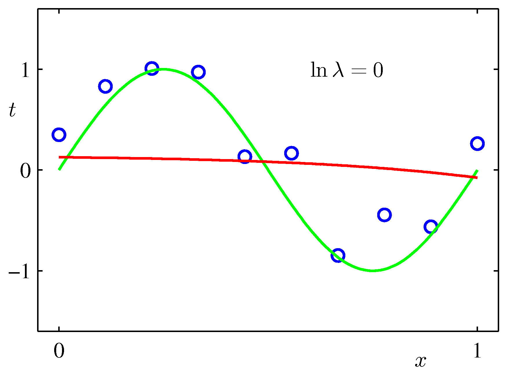
上記のPRMLの事例にある式で係数$\lambda$を固定して最小化を行った例($M=9$):$\lambda$が大きいと加重がきつくフィッティングされにくくなる。リッジ回帰では$\lambda$を手入力で与える必要がある。(下で試すscikit-learnではalphaという引数で指定)
import numpy as np
import random
import sklearn.linear_model as lm
import matplotlib.pyplot as plt

f_cos = lambda x: np.cos(2.0*x) # サンプルデータを作るためのベース関数

# データ数
n_tr = 10
x_max = 5.0 # xの範囲 [0, x_max]
x = np.linspace(0., x_max, n_tr)
y = f_cos(x) + np.random.randn(len(x))*0.3


# 単純な多項式近似
lrp = lm.LinearRegression()

for deg in [2,5,10]: # 最大べき
    power_matrix_x = np.vander(x, deg+1) # 計画行列の作成
    lrp.fit(power_matrix_x, y)
    # モデルの係数表示
    print('フィッティング関数の次数=' + str(deg))
    print('切片= ' + str(lrp.intercept_))
    print('係数= ' +  ' '. join(['%.3f' % c for c in lrp.coef_]))
    # 予測
    x_lrp = np.linspace(0., x_max*1.2, 100)
    y_lrp = lrp.predict(np.vander(x_lrp, deg+1))
    # 近似曲線の描画
    plt.plot(x_lrp, y_lrp)

# データの描画
plt.plot(x, y, "ob", ms=8)
plt.ylim(-2.0,2.0)

scikit-learnのリッジ回帰
マニュアルページ: https://scikit-learn.org/stable/modules/generated/sklearn.linear_model.Ridge.html
# リッジ回帰 alpha(正則化係数)の規定値は1.0
ridge = lm.Ridge(alpha=1.0)

for deg in [2,5,10]: # 最大べき
    ridge.fit(np.vander(x, deg +1), y) # リッジ回帰
    # 予測
    x_lrp = np.linspace(0., x_max*1.2, 100)
    y_lrp = ridge.predict(np.vander(x_lrp, deg+1))
    plt.plot(x_lrp, y_lrp,
            label='degree ' + str(deg))
    plt.legend(loc=2)
    # モデルの係数表示
    print('フィッティング関数の次数=' + str(deg))
    print('切片= ' + str(ridge.intercept_))
    print('  '. join(['%.5f' % c for c in ridge.coef_]))
    plt.plot(x, y , 'ok', ms=10)
    plt.title('Ridge Regression')

# サンプルデータのプロット
plt.ylim(-2.0,2.0)
plt.plot(x, y, "ob", ms=8)

Lasso回帰
ウェイトの項を単に絶対値$\frac{\lambda}{2}||{\bf w}||$にしたものをlasso回帰と呼ぶ。
model = lm.Lasso(alpha=0.01)
for deg in [2,5,10]: # 最大べき
    model.fit(np.vander(x, deg +1), y) # リッジ回帰
    # 予測
    x_lrp = np.linspace(0., x_max*1.2, 100)
    y_lrp = model.predict(np.vander(x_lrp, deg+1))
    plt.plot(x_lrp, y_lrp,
            label='degree ' + str(deg))
    plt.legend(loc=2)
    # モデルの係数表示
    # モデルの係数表示
    print('フィッティング関数の次数=' + str(deg))
    print('切片= ' + str(lrp.intercept_))
    print('係数' + ' '. join(['%.5f' % c for c in model.coef_]))
    plt.plot(x, y , 'ok', ms=10)
    plt.title('Lasso Regression')

# サンプルデータのプロット
plt.ylim(-2.0,2.0)
plt.plot(x, y, "ob", ms=8)

Lassoの場合、この程度のばらつきの場合だと、既定の加重係数(alpha=1.0)は大きすぎるようだ。また、データ数を多くしないと収束がわるという警告がでる。
全体として、次数を上げた場合、加重を含む最適化を行っているため、過学習が抑えられている。
係数alpha (上の式では$\lambda$)は外からあたえるパラメータであり、ハイパーパラメータと呼ばれる。
演習
データ作成のベース関数やデータ数、ハイパーパラメータ(正則化係数alphaやフィッティング関数の次数)を変えて振る舞いを確かめてみよう。