Frourier級数をpythonスクリプトで描画してみる

三角関数の重ね合わせ

周期が整数倍の三角関数を $$ f(x) = \sin(x) + \frac{1}{3}\sin(3x) + \frac{1}{5}\sin(5x) + \cdots $$ のように足し合わせると次の図のようになる。

# 最も簡単な描画例
%matplotlib inline
import numpy as np
import matplotlib.pyplot as plt

x = np.arange(-2.0*np.pi, 2.0*np.pi, 0.1)             # x軸方向のリスト（１次元配列）を用意
y = np.sin(x) + np.sin(3.0*x)/3.0 + np.sin(5.0*x)/5.0 # f(x)の計算 (yはxと同じ要素数のリストになる)

plt.plot(x,y)

[<matplotlib.lines.Line2D at 0x7fe1cdf54b00>]

一工夫をして、テキスト2.2の例１のような図を作ってみる

下の図は、テキスト2.2節の例1にある矩形波のフーリエ級数(p.67の(8)式)の最初の数項に相当する。(ただし、定数部分は除いた。)

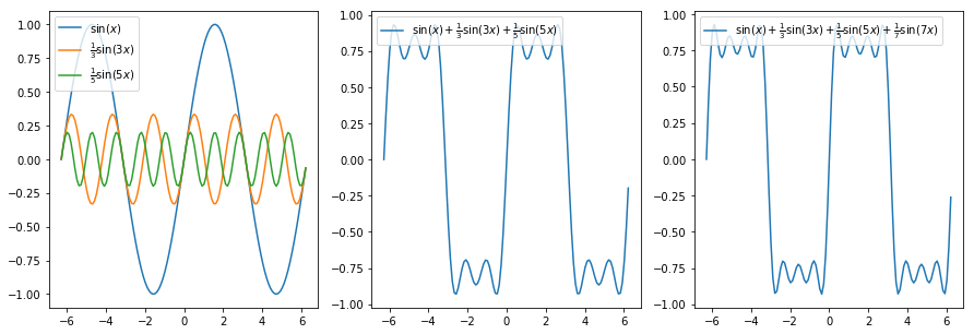
この図作成プログラム例 (冗長であるが、深く考えずに簡単に図示してみる場合にはこんな感じになるだろう。)

%matplotlib inline
import numpy as np
import matplotlib.pyplot as plt

xmin = -2.0*np.pi
xmax = 2.0*np.pi
fig = plt.figure(figsize=(15,5))
axes = fig.add_subplot(1,3,1)
x = np.arange(xmin, xmax, 0.1)
y_sin = np.sin(x)
y_sin3 = np.sin(3.0*x)/3.0
y_sin5 = np.sin(5.0*x)/5.0

axes.plot(x, y_sin, label="$\\sin(x)$")
axes.plot(x, y_sin3, label="$\\frac{1}{3}\\sin(3x)$")
axes.plot(x, y_sin5, label="$\\frac{1}{5}\\sin(5x)$")
plt.legend(loc='upper left')

axes2 = fig.add_subplot(1,3,2)
x = np.arange(xmin, xmax, 0.1)
y_sin = np.sin(x) + np.sin(3*x)/3 + np.sin(5*x)/5

axes2.plot(x, y_sin, label="$\\sin(x) + \\frac{1}{3}\\sin(3x) + \\frac{1}{5}\\sin(5x)$")
plt.legend(loc='upper left')

axes3 = fig.add_subplot(1,3,3)
x = np.arange(xmin, xmax, 0.1)
y_sin = np.sin(x) + np.sin(3*x)/3 + np.sin(5*x)/5 + np.sin(7*x)/7

axes3.plot(x, y_sin, label="$\\sin(x) + \\frac{1}{3}\\sin(3x) + \\frac{1}{5}\\sin(5x)+\\frac{1}{7}\\sin(7x)$")
plt.legend(loc='upper left')
plt.show()

もっと足し合わせて描画してみるページ

http://toyoki-lab.ee.yamanashi.ac.jp/~toyoki/lectures/appliedAnalysis2/plotSeries.html

このページは、JavaScriptで計算、図示している。ブラウザの右クリックでソースを表示してみるとプログラムがどのように書かれているかわかるだろう。

pythonで指定した次数までの数列和を表示する

単純に項の和を計算してみた例

# sec 2.2 4
%matplotlib inline
import numpy as np
import matplotlib.pyplot as plt

xmin = -2.0*np.pi
xmax = 2.0*np.pi
fig = plt.figure(figsize=(7,5))
axes = fig.add_subplot(1,1,1)
x = np.arange(xmin, xmax, 0.1)
y = 2/np.pi * (- np.cos(x) + np.cos(3.*x)/3 -np.cos(5*x)/5 + np.cos(7*x)/7 - np.cos(9*x)/9) \
     + 4/np.pi * (np.sin(2.*x)/2  + np.sin(6*x)/6  + np.sin(10*x)/10)
axes.plot(x, y)
plt.show()

共通部分を関数を用いて書く

いろいろな例に適用可能なように、係数$a_n$, $b_n$を計算する関数an(n), bn(n)の定義関数と数列和を計算・描画する関数を書いてみよう。

まず、表示する関数plotFourier(n)を書く。nは計算する最大項数。あとでan(n), bn(n)を定義する。

import numpy as np
import matplotlib.pyplot as plt

def plotFourierSeries(n):
    xmin = -2.0*np.pi
    xmax = 2.0*np.pi
    fig = plt.figure(figsize=(7,5))
    axes = fig.add_subplot(1,1,1)
    x = np.arange(xmin, xmax, 0.1)
    y = an(0)*np.ones(x.shape[0])
    for m in range(1,n+1,1):
        y = y+ an(m)*np.cos(m*x) + bn(m)*np.sin(m*x)
    axes.plot(x, y)
    plt.show()

項の係数の定義と描画

テキスト2.2節問題4の場合を例に作図してみる。$a_n$, $b_n$は次のように定義できる。 最後の行で、項数を指定して実行している。

import numpy as np
import matplotlib.pyplot as plt
# sec2.2 4
def an(n): # Fourier coefficient of cos
    if n%2 ==0:
        return 0.0
    else:
        a = 2.0/np.pi/n
        if (n+1)%4 ==0:
            return a
        else:
            return -a
def bn(n): # Frourier coefficient of sin
    if (n+2) %4 == 0:
        return 4.0/np.pi/n
    else:
        return 0.0

plotFourierSeries(10)

# sec2.2 7
import numpy as np
import matplotlib.pyplot as plt
# sec2.2 4
def an(n): # Fourier coefficient of cos
    if n ==0:
        return np.pi*np.pi/3.0
    else:
        a = 4.0/n/n
        if n%2 ==0:
            return a
        else:
            return -a
def bn(n): # Frourier coefficient of sin
    return 0.0

plotFourierSeries(100)

# 2.8 8 Fourier cosine transform (not good for including heavisede functions)
from sympy import integrate
from sympy.abc import x,k
F = integrate(x**2 * cos(k*x), (x, 0,1))
F

Piecewise((1/3, Eq(k, 0)), (sin(k)/k + 2*cos(k)/k**2 - 2*sin(k)/k**3, True))

# sine integral
import matplotlib.pyplot as plt
import numpy as np
import scipy.special
x = np.arange(-50, 50, 0.1)
y = scipy.special.sici(x)
plt.plot(x,y[0])
plt.show()