The harmonic oscillator is given by $$ \frac{dx}{dt} = \omega y,\quad \frac{dy}{dt} = -\omega x. $$ $x$ and $y$ represent the position and the velocity in the Newton equation of a mass under elastic force.
If we introduce a a complex variable $\psi = x- iy$, the equation leads to $$ \frac{d\psi}{dt} = (i\omega - \gamma)\psi, $$ where we add a dumping term. Its solution is easily obtained as $$ \psi (t) = \psi_0 e^{i\omega t -\gamma t} $$
Consider a nonlinear oscillater with a third-power term which yields a stable amplitude $|\psi|=1$: $$ \frac{d\psi}{dt} = i\omega \psi + (1- |\psi|^2)\psi\ . $$
Then, we introduce a mutual force entraining each other between two oscillators with : $$ \frac{d\psi_1}{dt} = i\omega_1 \psi_1 + (1- |\psi_1|^2)\psi_1 + D(\psi_2 - \psi_1) $$ $$ \frac{d\psi_2}{dt} = i\omega_2 \psi_2 + (1- |\psi_2|^2)\psi_2 + D(\psi_1 - \psi_2) $$
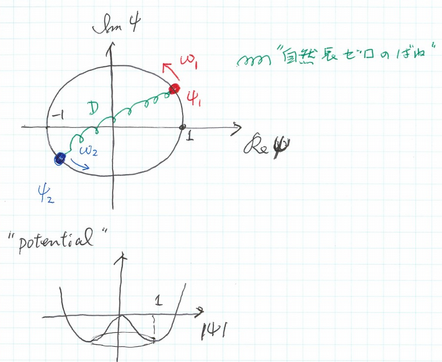
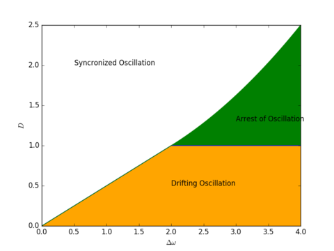
Our interest is on how these two oscillators' behavior depends on the difference of frequencies $\delta\omega = |\omega_1 - \omega_2 |$ and the interaction strength $D$. An analytical consideration leads to the following phase diagram which means the stationary state is divided into three regions.
For example, this is a simplest model to describe how the cells of heart muscle could oscillate synchronously even if their own frequence is slightly different from others.
まずは描画してみる
下のサブスライドにmatplotlibのアニメーション関数を使ったプログラムを掲載してあるので、相図を参考にパラメータを変えて実行してみてほしい。
パラメータは2つである。
- $\Delta \omega$ 2つの振動子の角振動数の違い(一方は$\omega=1$に固定)
- 差が大きいほど同期して動きにくくなる。
- $D$ 振動子間の結合係数
- 相手を自分のペースに引きずり込む効果の大きさを表す。
相図(再掲)
$D$と$\Delta\omega$の大きさにより振る舞いは3つの領域に分けられる。(このような図を相図(phase diagram)という。)
- matplotlibのanimationをインポート
- 微分方程式の右辺関数を定義
# coding: UTF-8
"""
  TDGL model of complex variables as a model of reaction-diffusion phenomena  described in chap. 15 of Ohta's textbook.

"""

import numpy as np
from scipy import integrate
from matplotlib import pyplot as plt
# from mpl_toolkits.mplot3d import Axes3D
from matplotlib import animation

def oscillator_deriv(x, t0, omega1=2., omega2= 1, D=1.5):
    """Compute the time-derivative of a coupled oscillator system. array of sets consisting of real part and imaginary part  """
    ampFac1 = 1.0 - (x[0]*x[0] + x[1]*x[1])
    ampFac2 = 1.0 - (x[2]*x[2] + x[3]*x[3])
    return [ampFac1*x[0] - omega1* x[1] + D*(x[2]- x[0]),
            ampFac1*x[1] + omega1* x[0] + D*(x[3]- x[1]),
            ampFac2*x[2] - omega2* x[3] + D*(x[0]- x[2]),
            ampFac2*x[3] + omega2* x[2] + D*(x[1]- x[3])]
アニメーションのための関数(メイン文から呼び出すと繰り返し実行される)
def animate(i):
    global start_t, x0, data4plot, t4plot, plot1, plot2

    start_t = start_t + width_ode
    # integration
    x_t = integrate.odeint(oscillator_deriv, x0, t, args=(omega1, omega2, D))
    # update data for plotting
    data4plot = np.vstack((data4plot, x_t))   # append new columns
    data4plot = data4plot[step:]            # delete "step" columns at the head
    # new values of the horizontal axis
    t4plot = np.linspace(start_t, start_t+width_plot, int(step*width_plot/width_ode))

    plt.xlim(min(t4plot), max(t4plot))
    plot1.set_xdata(t4plot)
    plot1.set_ydata(data4plot[:,0])
    plot2.set_xdata(t4plot)
    plot2.set_ydata(data4plot[:,2])
    x0 = x_t[-1]                     # initial value for the next calculation of ode
    return plot1, plot2
$D$, $\Delta\omega$をセットし、一枚目の図を作成、その後、アニメーション関数を実行
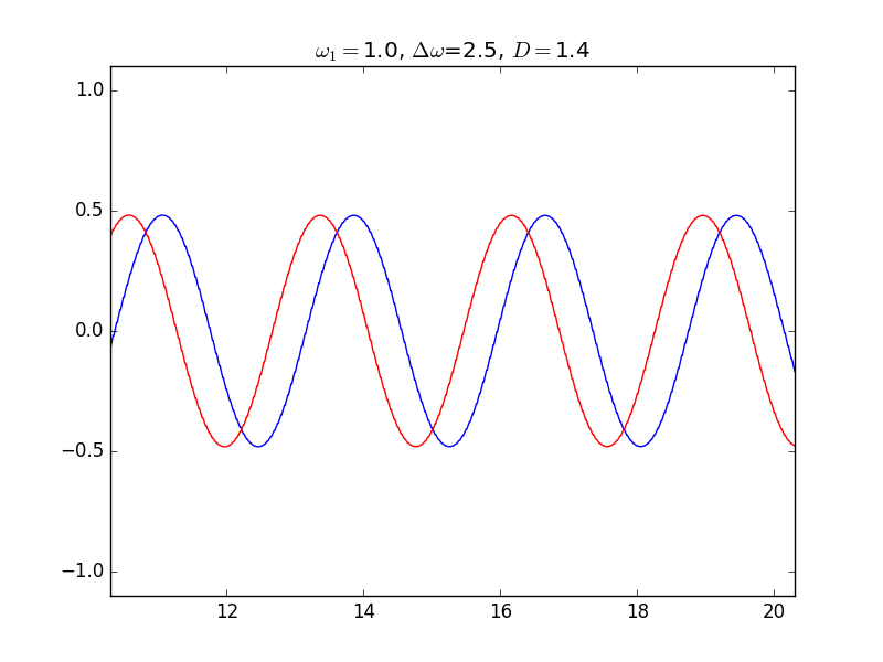
# parameters of the differential equation
omega1 = 1.0
deltaOmega = 2.5
D = 1.4
omega2 = omega1 + deltaOmega

# setting for animation
step = 5
width_ode = 0.05
width_plot = 10
t = np.linspace(0,width_ode,step)
x0 = [0.2, 0.2, 0.2, 0.2 ]  # starting vector

# Create new Figure and an Axes which fills it.
fig = plt.figure()

t4plot = np.linspace(0, width_plot, int(step*width_plot/width_ode))
data4plot = integrate.odeint(oscillator_deriv, x0, t4plot,
                             args=(omega1, omega2, D))  # ode calc.  for the first plot
plot1, = plt.plot([], [], 'b-')
plot2, = plt.plot([], [], 'r-')
plt.ylim(-1.1, 1.1)

x0 = data4plot[-1]
start_t =0

anim = animation.FuncAnimation(fig, animate,frames=1000, interval=20)
# anim.save('oscillator_xyz_t.mp4', fps=15, extra_args=['-vcodec', 'libx264']) #アニメーションを動画ファイルにする記述
plt.show()
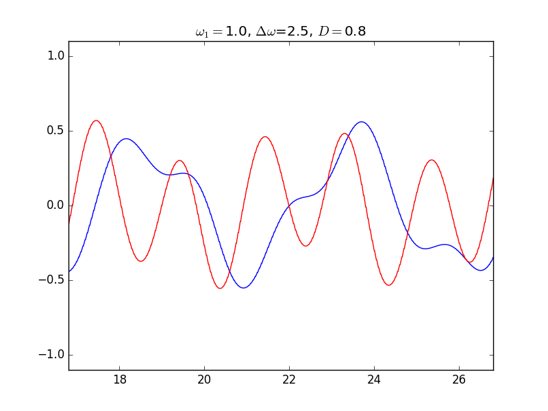
Drifting Oscillation (ドリフトモード)
$D$が小さくて、振動数の差が大きいので、影響し合いながらも、それぞれの振動数に基づく動きが主である。 青は$\omega=3.5$, 赤は$\omega=1.0$の振動子である。
GUI for the simulation of coupled nonlinear oscillation
The following is the simulation program implementing gui by using "tkinter", which is a somewhat classical but easy-to-use gui library. I could not run "animation" in matplotlib in the Tk frame, so I decided to introduce an button to update the system. The Tk create its own window and make the code run in the created window ("inline" statement of matplotlib does not work).
[note] The library name is "Tkinter" for python2 and "tkinter" for python3.
# coding: UTF-8
from Tkinter import *
import numpy as np
from scipy import integrate
from matplotlib.backends.backend_tkagg import FigureCanvasTkAgg
from matplotlib.figure import Figure
from matplotlib.lines import Line2D

class TwoTDGL:
    """
    class definition
    TDGL model of complex variables as a model of reaction-diffusion phenomena  described in chap. 15 of Ohta's textbook.
    """
    pause = False

    def oscillator_deriv(self, x, t0, omega1, omega2, D):
        """Compute the time-derivative of a coupled oscillator system. array of sets consisting of real part and imaginary part  """
        ampFac1 = 1.0 - (x[0]*x[0] + x[1]*x[1])
        ampFac2 = 1.0 - (x[2]*x[2] + x[3]*x[3])
        return [ampFac1*x[0] - omega1* x[1] + D*(x[2]- x[0]),
            ampFac1*x[1] + omega1* x[0] + D*(x[3]- x[1]),
            ampFac2*x[2] - omega2* x[3] + D*(x[0]- x[2]),
            ampFac2*x[3] + omega2* x[2] + D*(x[1]- x[3])]

    def __init__(self, D, delta, master):
        # create a container
        self.frame = Frame(master)
        self.fig = Figure()
        self.ax = self.fig.add_subplot(111)
        self.ax.set_ylim(-1.1, 1.1)
        self.ax.set_title("$\omega_1=$" + str(omega1) +", $\Delta\omega$=" + str(delta) + ", $D=$" + str(D))
        self.line1 = Line2D([],[], color='red')
        self.line2 = Line2D([],[], color='blue')
        self.ax.add_line(self.line1)
        self.ax.add_line(self.line2)
        self.canvas = FigureCanvasTkAgg(self.fig, master=master)
        self.canvas.get_tk_widget().pack()
        self.frame.pack(side="top")
        self.start_t = 0
        self.x0 = [0.2, 0.2, 0.2, 0.2 ]  # starting vector

    def run(self, D, delta):
        # set parameters of the differential equation and run
        self.omega1 = 1.0
        self.omega2 = omega1 + delta
        self.D = D
        self.step = 50
        self.width_ode = 0.5
        self.width_plot = 10
        self.update()

    def reset(self, D, delta):
        self.start_t =0
        setParams(D, delta)

    def update(self):
        self.t4plot = np.linspace(self.start_t, self.start_t + self.width_plot,
                                  int(self.step*self.width_plot/self.width_ode))
        self.data4plot = integrate.odeint(self.oscillator_deriv, self.x0, self.t4plot,
                                    args=(self.omega1, self.omega2,self.D))  # ode calc. for the first plot
        self.x0 = self.data4plot[-1]
        self.ax.set_xlim(self.start_t, self.start_t + self.width_plot)
        self.line1.set_data(self.t4plot,self.data4plot[:,0])
        self.line2.set_xdata(self.t4plot)
        self.line2.set_ydata(self.data4plot[:,2])
        self.im = 0
        self.canvas.show()
        self.start_t += self.width_plot

    def setParams(self, D, delta):
        self.D = D
        self.delta= delta
        self.omega1 = 1.0
        self.omega2 = self.omega1 + delta
        self.ax.set_title("$\omega_1=$" + str(omega1) +", $\Delta\omega$=" + str(delta) + ", $D=$" + str(D))

# end of CTDGL class definition

class controlFrame() :
    """
    control panel for starting, restarting and changing parameter values
    """
    def setupControlBox (self) :

        # control buttons
        self.controlBox.StartBtn = Button(self.controlBox,text=u"start", width=30)
        self.controlBox.StartBtn.bind("<Button-1>", self.startApp)

        # sliders for parameter setting
        self.controlBox.set_D = Scale(self.controlBox, from_=0.0, to=4.0, resolution=0.01, orient=HORIZONTAL, label="Interaction strength: D", length=500, command=self.changeParams)
        self.controlBox.set_delta = Scale(self.controlBox, from_=0.0, to=5.0, resolution=0.01, orient=HORIZONTAL, label="freq. difference: delta_omega", length=500, command=self.changeParams)
        self.controlBox.set_D.set(self.D) # initial value
        self.controlBox.set_delta.set(self.delta)

        # pack widgets in the control frame
        self.controlBox.StartBtn.pack()
        self.controlBox.set_D.pack()
        self.controlBox.set_delta.pack()
        return

    def startApp (self, ev) :
        D = self.controlBox.set_D.get()
        delta = self.controlBox.set_delta.get()
        self.simulationFrame.run(D,delta)
        self.controlBox.StartBtn.config(text=u"continue")

    def changeParams(self, ev):
        self.simulationFrame.setParams(self.controlBox.set_D.get(),
                                      self.controlBox.set_delta.get())

    # constructor of control panel
    def __init__(self, master=None, simulationFrame=None, D=0.5, delta=2.5):
        self.D = D
        self.delta =delta
        self.controlBox = Frame(master)
        self.setupControlBox()
        self.controlBox.pack(side="bottom")
        self.simulationFrame=simulationFrame

# end of controlBox class

if __name__ == "__main__" :
    # Create new Figure and an Axes which fills it.
    omega1 = 1.0
    delta_ini = 2.5
    D_ini = 1.4
    root = Tk()
    simF = TwoTDGL(D=D_ini, delta=delta_ini, master=root)
    app = controlFrame(master=root, simulationFrame=simF, D=D_ini, delta=delta_ini)
    root.mainloop()
Excitability (興奮性)を示す非線形方程式
神経膜の興奮性(閾値を超える刺激に対して平衡値から大きくずれ、ゆっくり元に戻る現象)を表す方程式としてホジキン・ハックスリー(Hodgkin-Huxley)方程式やそれを簡単化した南雲・フィッツヒュー(FitzHugh-Nagumo)方程式が有名である。
以下は、それを簡単化したもので太田のテキスト(太田隆夫、非線形の物理学、裳華房)に載っている。時間があれば数値計算して振る舞いを調べてみてほしい。
$$ \begin{eqnarray} \frac{du_1}{dt} & = & f(u_1) - v_1 + I_1 + k(u_2 -u_1)\\ \frac{dv_1}{dt} & = & b_1u_1 -\gamma_1v_1 + k(v_2 -v_1)\\ \frac{du_2}{dt} & = & f(u_2) - v_2 + I_2 + k(u_1 -u_2)\\ \frac{dv_2}{dt} & = & b_2 u_2 - \gamma_2 v_2 + k(v_1 - v_2) \end{eqnarray} $$where $$ f(u) = 10 u(u-1)(0.5-u) $$
Extension to oscillator chain described by one-dimensional differential equation
次の図のように振動子が1列に並んだ系を考えよう。
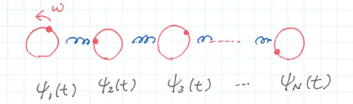
$\psi_n$に対する相互作用項は
$$ -D (\psi_n - \psi_{n-1}) + D(\psi_{n+1} - \psi_{n}) $$のように書かれる。振動子間の「距離」$h$を無限小にとり、$\psi_n$の$n$を連続変数$x$として$\psi (x)$について方程式を考える。上記の相互作用は
$$ Dh^2 \frac{1}{h} \left(\frac{\psi_{n+1} - \psi_{n}}{h} - \frac{\psi_n - \psi_{n-1}}{h}\right) \stackrel{h\to 0}{\rightarrow} D\frac{\partial^2 \psi (x)}{\partial x^2} $$のように2階微分として表される。(ただし、相互作用係数を新たに$D$とした。)
逆に、数値計算するときは、偏微分方程式の2階微分は、単純差分として
$$ \nabla^2 \psi \approx \psi_{n+1} + \psi_{n-1} - 2\psi_{n} $$を計算する。
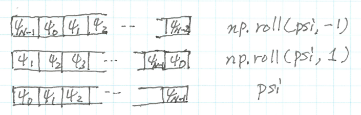
単純なpythonスクリプトにすると
for i in range(N):
    diff[i] = psi[i+1] + psi[i-1] - 2.*psi[i]
のように書くことができるが、先週試したように非効率である。かわりに、
diff = np.roll(psi,1) + np.roll(psi,-1) - 2.*psi
のようにnumpyの関数を利用すると高速に計算できる。roll()は配列を循環的に一つずらす(シフト)する関数である。つまり、上記のようにすると、周期的境界条件$\psi_{N} = \psi_{0}$を設定したことを意味する。固定周期境界や自由境界の場合は、端の設定を条件に合わせてセットする必要がある。
もし自由境界で解きたいなら $$ \psi_0 = \psi_1,\ \psi_{N-1} = \psi_{N-2} $$ のように、固定境界にするには、$\psi_0$と$\psi_{N-1}$を一定の値に保つようセットする。
import numpy as np
a = np.arange(10)
np.roll(a,-1)
a = np.random.rand(10)
print(a)
np.roll(a,1) + np.roll(a,-1) - 2.*a
プログラム例
説明は省略するが、少し一般化し係数を複素数とした方程式 $$ \frac{\partial \psi}{\partial t} = (1 + ic_0)\psi - (1+ic_2)|\psi|^2 \psi + (1+ic_1)\frac{\partial^2 \psi}{\partial x^2} $$ を数値計算し、アニメーション表示するプログラム例を掲げる。
境界条件により振る舞いが異なるので、それをメイン文でセットできるようにしてある。(独立したプログラムとするには、コマンドライン引数やGUIでパラメータをセットできるようにするのがよい。余裕があれば試してみてほしい。)
あまりかっこうのよいプログラムではないが、パラメータはメイン文でセットし、animate関数のなかではglobal宣言して値をうけとっている。(グローバル変数を関数内で扱う場合の例でもある。)
'''
Calculation and Animation for One-dimensional complex TDGL equation
(solved by simple Euler method.)

'''
%matplotlib auto
import numpy as np
from matplotlib import pyplot as plt
from matplotlib import animation
import sys
import math


size = 400
amp = np.zeros(size)    # used in the computing process as amplitudes
diff = np.array(amp, dtype=np.complex128)   # used as the Laplacian term

x = np.random.rand(size)
x = np.array(x, dtype=np.complex128)
y = np.array(x, dtype=np.complex128)
site_list = range(size)

def updateField(x_in, x_out, c0i =0.0 + 0.0j,  ci=1 + 0.6j, Di= 1 -1.0j, boundary="f"):
    DT = 0.002 # time step
    amp = np.absolute(x_in)
    amp = np.power(amp,2)
    diff[1:-1] = x_in[0:-2,] + x_in[2:]  - 2.0* x_in[1:-1]
    x_out[1:-1] = x_in[1:-1] + DT*(c0i - ci* amp[1:-1])*x_in[1:-1] + DT* Di * diff[1:-1]
    # periodic boundary condition
    if boundary=="periodic":
        x_out[0] = x_out[-2]
        x_out[-1] = x_out[1]
    elif boundary == "fixed":
        x_out[0] =0.2
        x_out[-1] = 0.2
    else:
        x_out[0] = 0.2
        x_out[-1] = x_out[-2]

fig = plt.figure(figsize=(7,4))
ax = fig.add_subplot(1,1,1)
ax.set_ylim(-2.0, 2.0)
plt_real_x, = ax.plot(site_list, np.real(x))
"""
animation function
"""
def animate(i):
    global x, y, c0i, ci, Di, size, boundary

    # integration
    for count in range(20):
        updateField(x, y, c0i, ci, Di, boundary)
        updateField(y, x, c0i,  ci, Di, boundary)

    # update data for plotting
    # crgb =  (np.angle(x) + math.pi)/2.0/math.pi
    plt_real_x.set_data(site_list, np.real(x))
    return [plt_real_x]


if __name__ == '__main__':
    # parameters
    c0 = -0.5
    c1 = 0.0
    c2 = 0.6
    initial_condition = 1 # 1 = random, otherwise = [0]
    boundary = "free"   # "free", "fixed" or  "periodic"

    c0i = 1.0 + c0*1.0j
    Di = 1.0  + c1*1.0j
    ci = 1.0 + c2*1.0j
    plt.title("$c_0=" + str(c0) + ", c_1=" + str(c1) + ", c_2="
              + str(c2) + "$, boudary=" + boundary)
    # initial configuration
    if initial_condition == 1:
        for n in range(size):
            x[n] = 0.01*(np.random.rand() -0.5 + (np.random.random() - 0.5)* 1.0j)
    else:
        for n in range(size):
            x[n] = 0.0 + 0.0j

    anim = animation.FuncAnimation(fig, animate,
                               frames=1000, interval=10)
    # anim.save('ctdgl2d.c1_1.0_c2_0.6.mp4', fps=15, extra_args=['-vcodec', 'libx264'])
    # anim.save('oscillator_xyz_t.gif', writer='imagemagick',  fps=30)
    plt.show()
パラメータの設定例
- c0=0.5, c1 =0., c2=0.6, initial_condition=0, boundary="free": "励起波"
- c0=0.5, c1 =0., c2=0.6, initial_condition=0, boundary="free": "左右の波の「干渉」"
- c0=0.5, c1=2.0, c2=-0.2, initial_condition=1, boundary="periodic": 長期的には「孤立波」的な振る舞い
メイン文のなかのパラメータをこのような値にセットして振る舞いを確かめてみてほしい。
古い資料だが、次のページにもう少し詳しい事例が紹介されている。
https://toyoki-lab.ee.yamanashi.ac.jp/~toyoki/lectures/complexSys/ctdgl_pde/ctdgl_pde.html